Tutorial
Folder: examples/tutorial
This folder contains the smallest TARSA examples that still use real meteorology. For a first run, start with minimal_code.jl. Use 01_run_point_source.jl when you want the same Etna case saved as tutorial_plume.nc for the GIF step in 02_make_plume_gif.jl.
Purpose
This tutorial keeps the workflow short:
- get ERA5 automatically,
- load it into
TARSA.InputFields, - place a point source on the ERA5 grid,
- run it through
AerosolTracer, - save a GIF-ready plume NetCDF,
- optionally render a GIF of the plume.
The source is deliberately simple so the main idea stays clear: you can work directly with real ERA5 winds, density, and vertical structure without writing a large driver script.
What this tutorial uses
The checked-in tutorial case uses:
| Setting | Value |
|---|---|
| Region | Mediterranean box around Etna |
| Requested box | lon = 12-18, lat = 34-40 |
| Date | 2024-04-01 to 2024-04-02 |
| Source type | steady point source |
| Source location | near Etna (15.0, 37.75) |
| Emission rate | 8 kg/s |
| Injection height | 2500 m |
| Vertical spread | sigma_z = 600 m |
| Tracer | AerosolTracer(radius_m=0.11e-6, density_kg_m3=1700.0) |
| Solver | explicit :dst_koren_rk3 |
| Tutorial runtime | two requested ERA5 days (48 hourly steps) |
Before you run
You need:
- Julia with the TARSA project instantiated
- internet access on the first run, unless the ERA5 files are already cached
ERA5 download requires Copernicus credentials, either through ~/.cdsapirc or through the CDSAPI_URL and CDSAPI_KEY environment variables. The exact setup is described in Guide / Data Access.
The repository also ships the exact tutorial ERA5 subset in examples/tutorial/data/:
era5_2024_04_01_levels.ncera5_2024_04_01_surface.ncera5_2024_04_01_precip.nc
This means a new user can usually run the tutorial immediately without waiting for a fresh Copernicus request. If you remove these files and force a new download, budget roughly 10 minutes for the Copernicus transfer and about 1 minute for the actual TARSA tutorial computation.
Pipeline
Download or reuse ERA5
The tutorial begins by resolving the meteorology files. The repository already includes the required tutorial files in examples/tutorial/data/, so they are normally reused immediately. If they are missing, TARSA downloads them automatically.
Core step:
levels_file, surface_file, precip_file, _ = TARSA.prepare_input_data(
    CASE.lat_min,
    CASE.lat_max,
    CASE.lon_min,
    CASE.lon_max,
    CASE.year,
    CASE.month,
    CASE.days;
    download_cams=false,
    data_dir=DATA_DIR,
)
Load meteorology into TARSA
Once the files exist, the tutorial uses the high-level loader:
input = TARSA.load_input_data(levels_file, surface_file)This creates a single InputFields object that carries the meteorology, coordinates, and grid spacing.
Build a point source on the ERA5 grid
The source is built with:
emissions = TARSA.zero_emissions(input)
TARSA.add_point_source!(
    emissions,
    input,
    SOURCE.lon,
    SOURCE.lat;
    rate_kg_s=SOURCE.rate_kg_s,
    injection_height=SOURCE.injection_height_m,
    sigma_z=SOURCE.sigma_z_m,
)
This is the key tutorial step. The source is defined in physical coordinates and TARSA maps it directly onto the loaded ERA5 grid.
Configure and run the aerosol solver
The actual simulation path is short:
- Load the aerosol process inputs:
aerosol_inputs = TARSA.load_aerosol_inputs(
    levels_file,
    precip_file;
    surface_file=surface_file,
)- Build the solver configuration:
solver = TARSA.ExplicitSolver(
    cfl=SOLVER.cfl,
    scheme=SOLVER.scheme,
    dt=SOLVER.dt_seconds,
)- Turn meteorology and emissions into an aerosol simulation object:
sim = TARSA.build_aerosol_simulation(
    input,
    emissions;
    aerosol=AEROSOL,
    aerosol_inputs=aerosol_inputs,
    processes=TARSA.AerosolProcesses(
        sedimentation=true,
        wet_deposition=TARSA.WetDeposition(),
        dry_deposition=TARSA.DryDeposition(lai=fill(2.0f0, input.Nx, input.Ny)),
    ),
    solver=solver,
    lateral_bc=:neumann0,
    bottom_bc=:neumann0,
)- Run the model:
mixing_ratio = TARSA.run!(sim)This is still the main high-level TARSA pattern to remember, now using the public aerosol API directly.
Write the plume output
The only extra step beyond minimal_code.jl is saving the plume file that the GIF script expects:
TARSA.save_results(
    OUTPUT_FILE,
    input,
    mixing_ratio,
    emissions;
    template_file=levels_file,
    variables=["concentration"],
    save_emissions=false,
)
This writes:
out/tutorial_plume.nc
The NetCDF file is created from the ERA5 template and adds the simulated concentration field plus the source and aerosol metadata used by the plotting step.
Make the GIF
After the tutorial run, you can render the plume animation with:
julia --project=. examples/tutorial/02_make_plume_gif.jlThis writes:
out/tutorial_plume_surface.gif
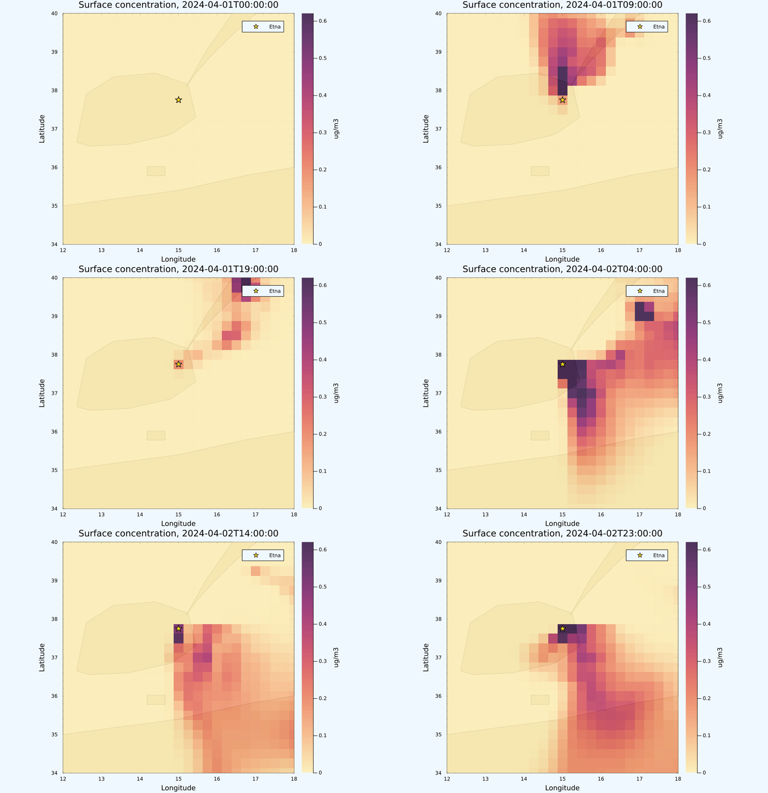
The GIF shows the evolving near-surface concentration over the tutorial domain and marks the source location.
How to run
For the shortest path:
julia --project=. examples/tutorial/minimal_code.jlThis writes:
examples/tutorial/out/quickstart_etna.nc
For the tutorial run used for the GIF:
From the repository root:
julia --project=. examples/tutorial/01_run_point_source.jlOr from inside examples/tutorial/:
julia --project=../.. minimal_code.jl
julia --project=../.. 01_run_point_source.jl
What to expect
This is a real-meteorology run, so the plume does not follow an idealized straight path. Its transport depends on the ERA5 winds in the chosen time window.
What should stay true:
- the source is anchored near the chosen volcano point,
- the final plume shifts downwind relative to the source,
tutorial_plume.nccontains nonzeroconcentrationvalues.
How to adapt this tutorial
For the shortest case edits, change the parameter values near the top of examples/tutorial/minimal_code.jl.
For examples/tutorial/01_run_point_source.jl, the quickest edits are:
CASE: change the date window or domain,SOURCE: change location, rate, injection height, or vertical spread,AEROSOL: change particle radius or density,SOLVER: changecfl, scheme, or model time step.
Good first adaptations:
- move the source to a different volcano or industrial stack,
- shrink the domain for a faster first run,
- edit
CASE.daysto request a shorter or longer period, - vary
AEROSOL.radius_morAEROSOL.density_kg_m3, - test how plume spread changes with a different
sigma_z.
If you want the same tutorial pattern with a surface source instead of an elevated plume, use:
emissions = TARSA.zero_emissions(input)
TARSA.add_ground_source!(
    emissions,
    input,
    SOURCE.lon,
    SOURCE.lat;
    rate_kg_s=SOURCE.rate_kg_s,
)
If you want full control, build the 4D volumetric emissions array directly:
emissions = TARSA.build_custom_emissions(input) do E, input
    dz = TARSA.calculate_dz_full(input.geopotential)
    i = argmin(abs.(input.longitude .- SOURCE.lon))
    j = argmin(abs.(input.latitude .- SOURCE.lat))
    rate_t = fill(Float32(SOURCE.rate_kg_s), input.Nt)

    for t in 1:input.Nt
        volume = input.dx[i, j] * input.dy[i, j] * dz[i, j, 1, t]
        E[i, j, 1, t] = rate_t[t] / volume
    end
end