Manufactured Gaussian plume verification
Purpose
This verification case compares TARSA against an analytical Gaussian plume solution in a uniform flow. It is used to verify the coupled 3-D advection + turbulent diffusion behaviour in a controlled, idealised configuration before moving to real-case validations.
The Gaussian runs use the same default numerics as ETEX and the demo cases:
- Advection: DST–Koren (TVD MUSCL reconstruction) with a Koren–Sweby limiter
- Time integration: SSP-RK3
- Vertical diffusion: implicit (column-wise Thomas solver)
- Splitting: second-order Strang splitting of advection and vertical diffusion
Configuration
We consider a Cartesian domain
\[[-1500,1500]\times[-400,400]\times[0,100]~\mathrm{m},\]
discretised on a uniform grid. The current reference configuration in validation_gaussian_multiresolution.jl uses 121×11×61 cells ($\Delta x=25~\mathrm{m}$, $\Delta y=80~\mathrm{m}$, $\Delta z\approx1.67~\mathrm{m}$).
The wind is purely along-wind ($u_x=5~\mathrm{m\,s^{-1}}$, $u_y=u_z=0$) and the turbulent diffusivity is constant ($K_z=0.05~\mathrm{m^2\,s^{-1}}$ by default). A compact volumetric source is placed in the central grid cell and scaled to match the analytical emission rate $Q$.
Boundary conditions follow the manufactured-test setup:
- lateral boundaries treated as open ($C=0$),
- reflecting lower boundary at $z=0$ (zero flux), consistent with the analytical image solution.
Starting from $C=0$, TARSA is integrated with the Strang-split DST–Koren + SSP-RK3 configuration. The time step is chosen from the CFL restriction; for the reference grid and wind speed a stable choice corresponds to $\mathrm{CFL}\approx 0.5$. The results below are reported at the end of the integration window $T_{\mathrm{end}}=900~\mathrm{s}$.
Results
The figures below reproduce the key diagnostics for this case.
Horizontal maps and normalised error
Map figure PDF: 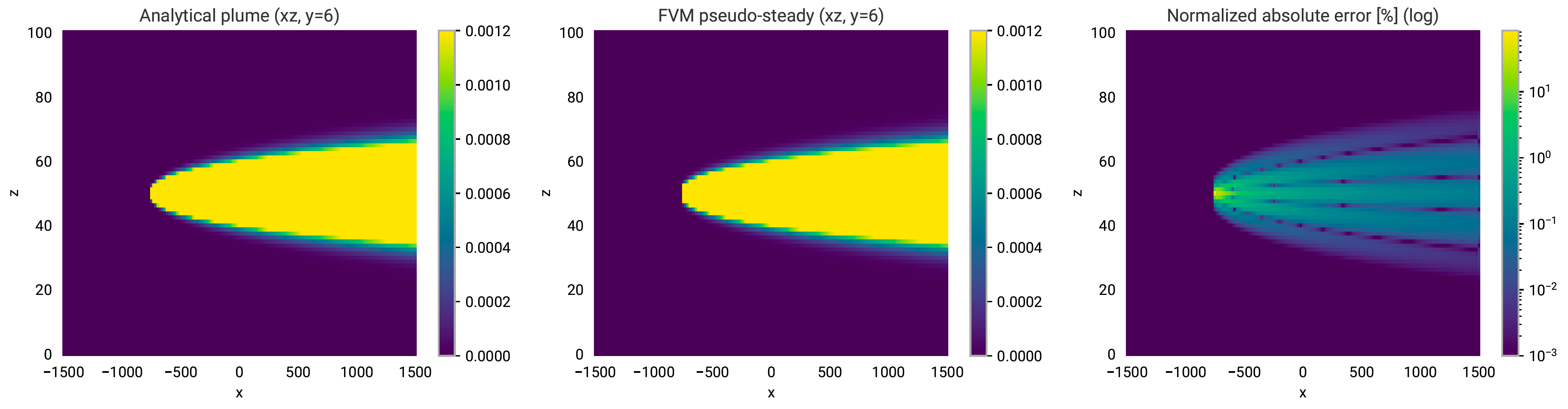
Left: analytical solution; middle: TARSA solution; right: normalised absolute error
\[\frac{C_{\mathrm{plume}}-C_{\mathrm{FVM}}}{\max(C_{\mathrm{FVM}})}.\]
Cell-wise scatter (log–log)
Cell-wise comparison between analytical and TARSA solutions using $N=5551$ evaluated grid points. Both axes are logarithmic.
Scatter figure PDF: 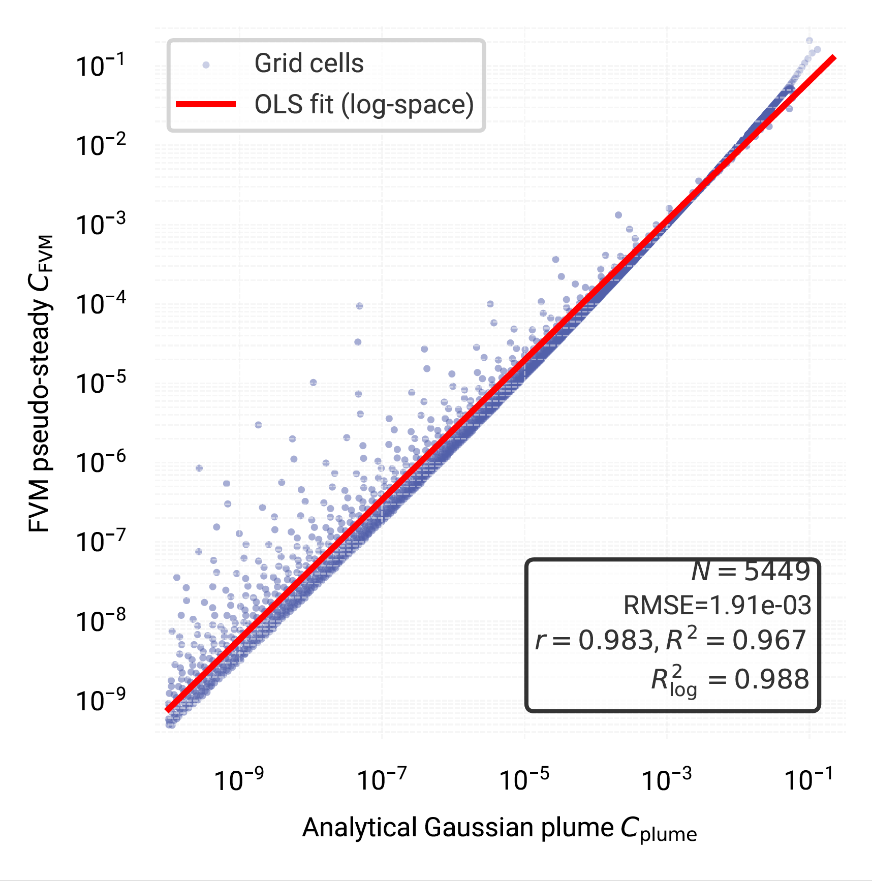 {width=50%}
For the reference grid, the agreement is high over a wide dynamic range (points close to the 1:1 line). For this run, Pearson correlation is $r=0.982$ ($R^2=0.964$), with a small fractional bias (FB$=0.004$), a normalised mean square error NMSE$=0.285$, and a high figure of merit FM$=0.973$. The remaining spread at the highest values is primarily due to (i) discretisation near the emission cell and (ii) TVD limiting in the DST–Koren reconstruction, which introduces a small amount of limiter-related diffusion in regions of strong gradients to maintain boundedness. Deviations at extremely small concentrations correspond to cells where both solutions approach machine precision and log-space diagnostics become sensitive to roundoff.
Grid sensitivity
To assess sensitivity to spatial resolution, the multi-resolution script repeats the Gaussian plume experiment on coarse, reference and fine grids while keeping the physical domain and forcing identical. The agreement improves monotonically with resolution.
| Grid | $N_x\times N_y\times N_z$ | $N$ | $r$ | $R^2$ | FB | NMSE | REL$_{L2}$ |
|---|---|---|---|---|---|---|---|
| coarse | $81\times 9\times 41$ | 2501 | 0.9766 | 0.9538 | 0.0072 | 0.3845 | 0.2325 |
| reference | $121\times 11\times 61$ | 5551 | 0.9820 | 0.9643 | 0.0041 | 0.2845 | 0.1952 |
| fine | $161\times 13\times 81$ | 9801 | 0.9850 | 0.9702 | 0.0028 | 0.2317 | 0.1740 |
Why this case matters
- provides an analytical reference for the advection–diffusion core
- serves as a regression test for the default explicit numerics (DST–Koren + SSP-RK3 + Strang + implicit vertical diffusion)
- underpins the differentiability / gradient-check experiments that reuse the same manufactured configuration
How to run
Scripts
Folder: validation/GAUSSIAN
Main scripts:
validation/GAUSSIAN/validation_gaussian_explicit.jlvalidation/GAUSSIAN/validation_gaussian_multiresolution.jlvalidation/GAUSSIAN/validation_gaussian_plot.py
validation_gaussian_explicit.jl
- defines analytical plume solution (including ground reflection)
- runs TARSA forward with the explicit Strang-split configuration
- writes fields and metrics consumed by the plotting script
validation_gaussian_multiresolution.jl
- runs the same configuration on
coarse,reference,finegrids - writes a summary CSV (e.g.
gaussian_multiresolution_stats.csv) with metrics:R,R2,FB,NMSE,FM,RMSE,REL_L2
validation_gaussian_plot.py
- produces the map triptych and scatter plot PDFs
Run
julia --project=. validation/GAUSSIAN/validation_gaussian_multiresolution.jl
julia --project=. validation/GAUSSIAN/validation_gaussian_explicit.jl
python validation/GAUSSIAN/validation_gaussian_plot.py --no-show