Regularised TVD limiter validation
Purpose
This case validates the cubic-Hermite regularisation of the Koren TVD limiter used by the explicit DST-Koren transport core, and documents a small source-position sensitivity diagnostic used to check whether the regularisation reduces limiter-induced gradient noise.
It answers five practical questions:
- Does the smoothed limiter stay inside the Sweby TVD admissible region?
- Do the Hermite patches join with the intended
C0andC1continuity? - Does the analytic limiter derivative agree with finite differences away from the exact branch knots?
- Are the default smoothing widths robust to parameter stress tests?
- Does the regularised limiter reduce sensitivity roughness without materially changing the forward transport response?
This page isolates the limiter itself. For end-to-end gradient behaviour of the full transport solver, see Gradient / AD experiments.
Relation to the production solver
The production explicit solver uses the smoothed Koren limiter in src/numerics/FVM_explicit_common.jl through:
koren_limiter(r)koren_limiter_and_grad(r)
with checked-in default widths
\[\delta_1 = 0.02,\qquad \delta_2 = 0.05.\]
The validation folder re-implements the same limiter logic in a small standalone form so that the TVD and smoothness properties can be tested directly. The legacy delta0 parameter is retained in the validation configuration for compatibility with older sweeps, but the production limiter no longer applies a Hermite patch at r = 0.
Limiter construction
The unsmoothed Koren limiter is
\[\phi_{\mathrm{Koren}}(r)= \begin{cases} 0, & r \le 0, \\ 2r, & 0 < r < \tfrac14, \\ \dfrac{1+2r}{3}, & \tfrac14 \le r < \tfrac52, \\ 2, & r \ge \tfrac52. \end{cases}\]
The regularised TARSA variant replaces the two active Koren branch joins with cubic-Hermite patches:
\[r \in \left[\frac{1}{4}-\delta_1,\;\frac{1}{4}+\delta_1\right],\]
and
\[r \in \left[\frac{5}{2}-\delta_2,\;\frac{5}{2}+\delta_2\right].\]
The patch endpoints are chosen to match both value and slope of the neighbouring linear branches, so the resulting limiter is C1 at the active branch transitions while preserving the original Koren shape outside the small transition intervals.
The corner at r = 0 is intentionally left classical. For a strict Sweby limiter, phi(r) = 0 for r <= 0 and 0 <= phi(r) <= 2r for r > 0. A finite Hermite patch that starts with zero slope at r = 0 and rejoins the high-resolution branch phi = 2r at finite positive r must catch up inside the patch; in the previous cubic construction this introduced a local derivative overshoot. Leaving the r = 0 TVD corner classical avoids that artificial spike while still smoothing the active Koren branch transitions at r = 1/4 and r = 5/2.
For a valid geometry, the widths must satisfy:
\[\delta_1 > 0,\qquad \delta_2 > 0,\qquad \frac{1}{4}-\delta_1 > 0,\qquad \frac{1}{4}+\delta_1 < \frac{5}{2}-\delta_2.\]
What is checked
The validation scripts test the differentiable limiter against the same properties that matter for high-resolution finite-volume transport:
- Bounds:
0 <= phi(r) <= 2 - Sweby ratio condition:
phi(r)/r <= 2forr > 0 - Consistency:
phi(1) = 1 - Continuity diagnostics: numerical
C0andC1checks near every patch boundary - Exact interface matching: endpoint value and slope residuals at every Hermite join
- Monotonicity: dense-grid nondecreasing behaviour over a broad
rinterval - Derivative consistency: analytic derivative against centered finite differences
- Parameter robustness: randomized and structured sweeps over smoothing widths
- Sensitivity roughness: a source-position sweep comparing classical Koren, regularised Koren, van Leer, and first-order upwind
Two complementary TVD checks are used:
- an analytic certificate that checks cubic patch extrema directly through critical points
- a dense sampling check over large
rranges as a second independent numerical guard
Results
Default TARSA smoothing widths
For the production default
\[(\delta_1,\delta_2) = (0.02, 0.05),\]
the strict validation script reports:
- analytic TVD certificate:
ok = true - dense-grid TVD check:
ok = true min(phi) = 0max(phi) = 2max(phi - 2r) = 0phi(1) = 1
The continuity diagnostics for the default configuration are:
- numerical
C0max jump at retained patch boundaries:3.999999831361123e-8 - numerical
C1max jump at retained patch boundaries:3.333333331578814e-7 - exact interface value jump:
0 - exact interface slope jump:
0
The dense monotonicity check reports:
- minimum increment over the sampled grid:
0
This means the checked default limiter remains bounded, TVD-safe, and smoothly patched at the two retained regularised branch locations. The r = 0 corner remains nonsmooth by design.
AD-oriented strong checks
The stronger validation script adds derivative and near-knot stress tests. In the checked run:
209adversarial near-knot samples passed the TVD inequalities300analytic-vs-finite-difference gradient checks passed160randomized geometry-valid parameter sets passed the strong TVD/interface checks
These results are the direct limiter-level evidence that the differentiable construction is suitable for tangent, adjoint, and autodiff workflows at the retained Hermite branch transitions. They do not prove global differentiability of the full transport model, and they do not remove nonsmoothness at r = 0 or at degenerate stencils where the downwind gradient used in the ratio is near zero.
Source-position sensitivity diagnostic
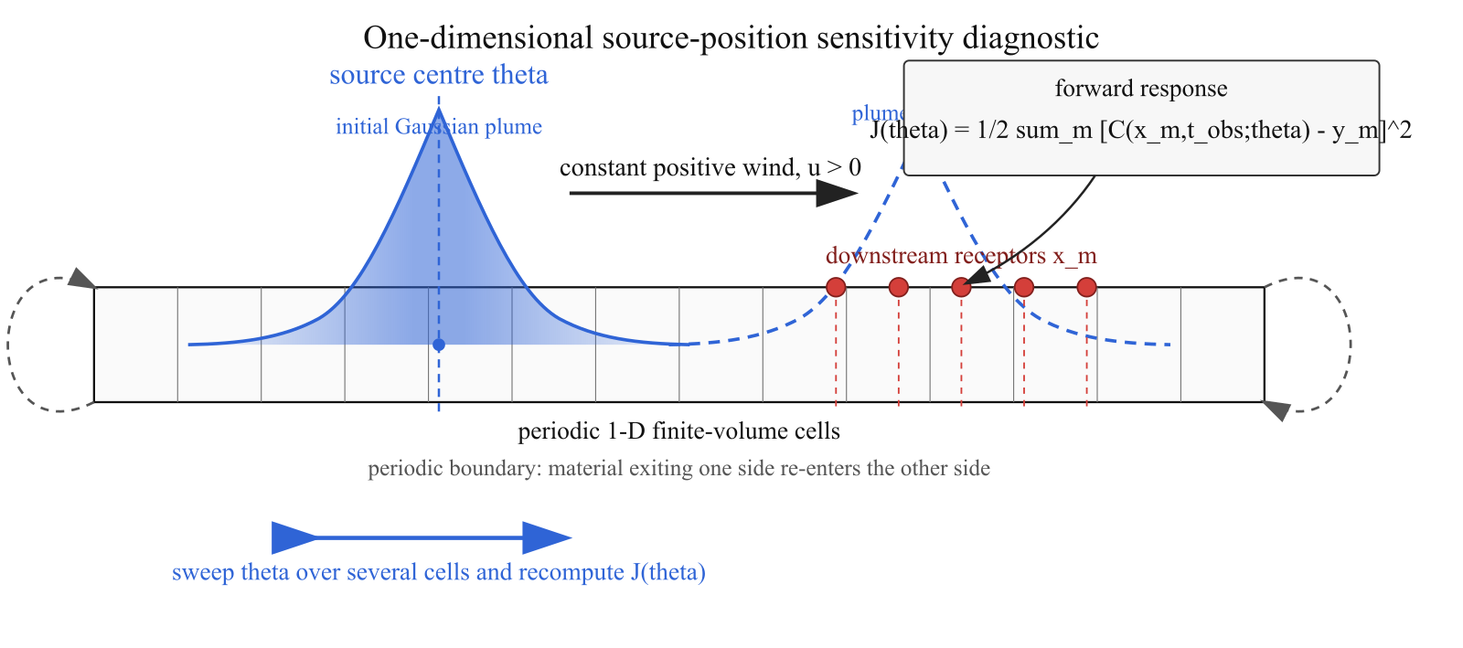
The limiter-level checks above certify TVD admissibility and local patch smoothness. A separate diagnostic in validation/TVD_limiter/regularised_koren_diagnostic.jl tests the consequence for a small transport response. It uses a one-dimensional periodic passive-advection problem with constant positive velocity, no deposition, and an initial Gaussian plume. The control parameter is the source centre theta.
Here the forward response means the scalar quantity produced by running the forward transport model for a given source position. It is not a gradient and it is not an adjoint quantity. For each sampled source position, the model is run forward to the observation time, the transported concentration is sampled at a small set of downstream receptors, and those modelled receptor values are compared with fixed synthetic observations. The diagnostic uses the least-squares response
\[J(\theta) = \frac12 \sum_m \left[C(x_m,t_{\mathrm{obs}};\theta) - y_m\right]^2,\]
where C(x_m,t_obs;theta) is the forward-model concentration at receptor x_m and observation time t_obs, and y_m are synthetic observations generated from a nearby reference source position. Comparing J(theta) between limiters tests whether changing the limiter changes the actual forward transport result. A small relative forward-response change means that the limiter modification affects the diagnostic sensitivity without materially changing the predicted plume response.
The schematic below summarises the experiment. The dashed grey wrap-around arrows outside the grid indicate the periodic boundary condition: material leaving the right edge re-enters from the left edge, and vice versa. A Gaussian initial condition is centred at the control position theta on a periodic one-dimensional finite-volume grid. The plume is transported to the right by a constant positive wind. At the observation time, concentrations are sampled at fixed downstream receptor locations x_m; these values are then combined into the scalar response J(theta).
The sensitivity
\[g_i = \frac{dJ}{d\theta}(\theta_i)\]
is evaluated with the same centred finite-difference method for every limiter.
The diagnostic compares four schemes:
- classical piecewise Koren,
- regularised Koren with the
r = 0corner left classical and Hermite patches atr = 1/4andr = 5/2, - van Leer, a published smooth TVD limiter for
r > 0, - first-order upwind.
Gradient noise is quantified with three discrete roughness measures on the sampled sensitivity curve:
\[\max|\Delta g| = \max_i |g_{i+1}-g_i|,\]
the largest adjacent gradient jump;
\[\sum|\Delta g| = \sum_i |g_{i+1}-g_i|,\]
the total variation of the sampled gradient; and
\[\sum|\Delta^2 g| = \sum_i |g_{i+1} - 2g_i + g_{i-1}|,\]
a second-difference roughness measure that highlights rapid changes in the gradient slope.
The figure below reports these roughness metrics normalised by the corresponding classical Koren value. Values below one indicate lower sensitivity roughness than the classical piecewise limiter. The last panel reports the maximum relative change in the scalar forward response relative to classical Koren.
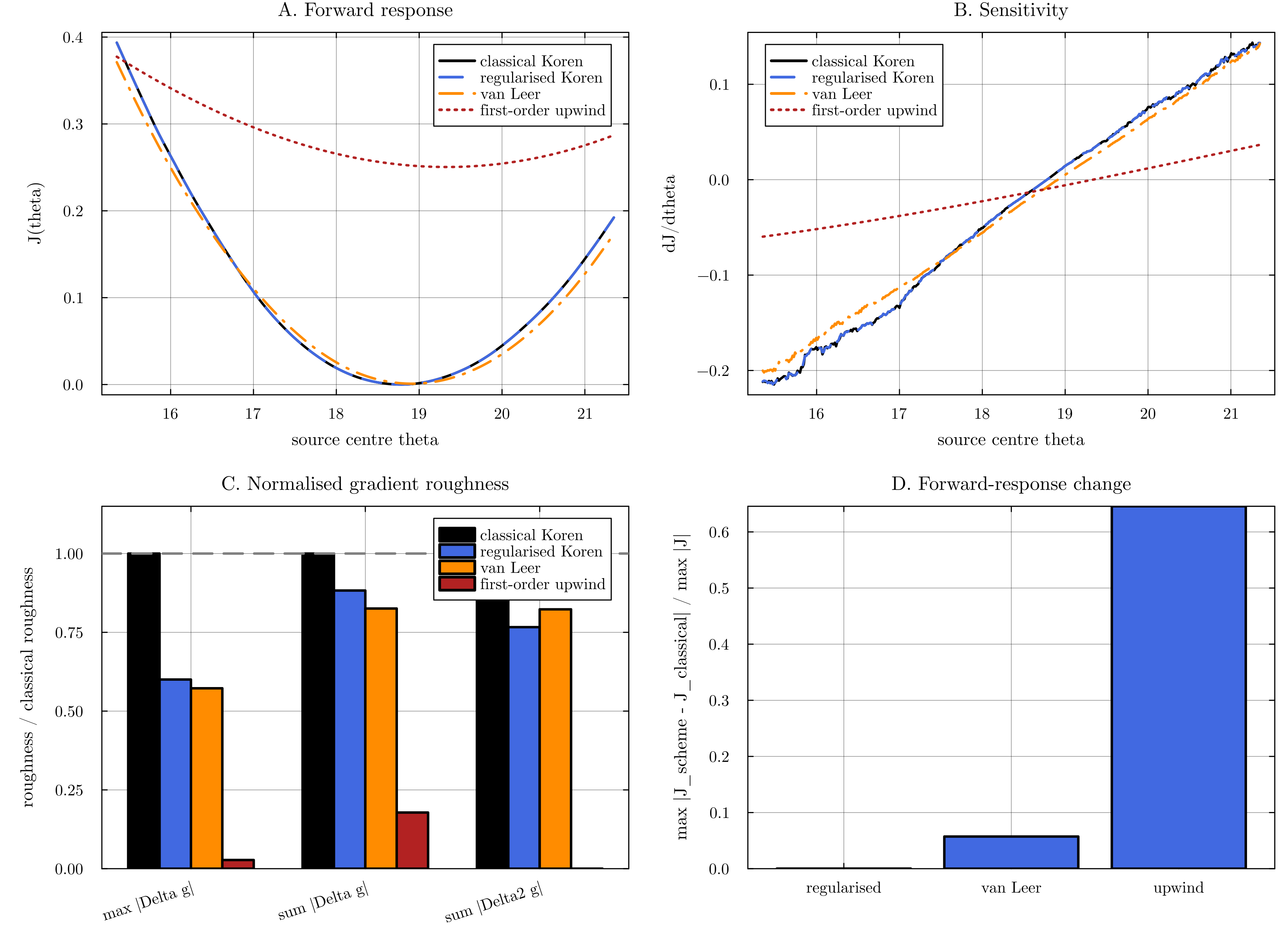
For the checked diagnostic run, the absolute metrics were:
| scheme | $\max \lvert \Delta g \rvert$ | $\sum \lvert \Delta g \rvert$ | $\sum \lvert \Delta^2 g \rvert$ | max relative forward-response change |
|---|---|---|---|---|
| classical Koren | 9.9867e-3 | 5.4067e-1 | 6.5527e-1 | 0 |
| regularised Koren | 5.9943e-3 | 4.7722e-1 | 5.0224e-1 | 1.5430e-4 |
| van Leer | 5.7168e-3 | 4.4635e-1 | 5.3926e-1 | 5.7265e-2 |
| first-order upwind | 2.7523e-4 | 9.6308e-2 | 1.0429e-4 | 6.4569e-1 |
This comparison is useful because it separates sensitivity smoothness from forward accuracy. First-order upwind gives the smoothest sensitivity, but only by introducing strong numerical diffusion and changing the forward response by about 65% in this diagnostic. Van Leer reduces some first-difference roughness but changes the forward response by about 5.7%. The regularised Koren limiter reduces all three gradient roughness measures while keeping the forward response nearly unchanged, with a maximum relative response difference of about 1.5e-4.
The scientific conclusion is therefore deliberately limited: this diagnostic provides evidence that regularising the active Koren branch transitions reduces limiter-induced sensitivity noise for this trajectory, without materially changing the forward transport response. It is not a proof that the full TARSA model is globally smooth.
Active smoothing-width sweep
The active regularisation widths are delta1 and delta2. They are half-widths of the Hermite transition patches around the two retained Koren branch points:
\[\delta_1:\quad r \in \left[\frac{1}{4}-\delta_1,\;\frac{1}{4}+\delta_1\right],\]
and
\[\delta_2:\quad r \in \left[\frac{5}{2}-\delta_2,\;\frac{5}{2}+\delta_2\right].\]
For example, delta1 = 0.02 gives a first transition patch over r in [0.23, 0.27], while delta2 = 0.15 gives a second transition patch over r in [2.35, 2.65]. Increasing a width spreads the corresponding branch transition over a larger range of gradient ratios. This can reduce abrupt changes in the local discrete Jacobian, but if the patch is too wide it can also alter the forward transport response.
The heatmap below sweeps delta1 and delta2 in the source-position diagnostic. Each cell is one pair of smoothing widths. Darker colours indicate lower values of the plotted metric. Panels A-C show the same gradient roughness diagnostics described above, and panel D shows the maximum relative forward-response change relative to classical Koren. The white star marks the lowest second-difference roughness in the tested grid.
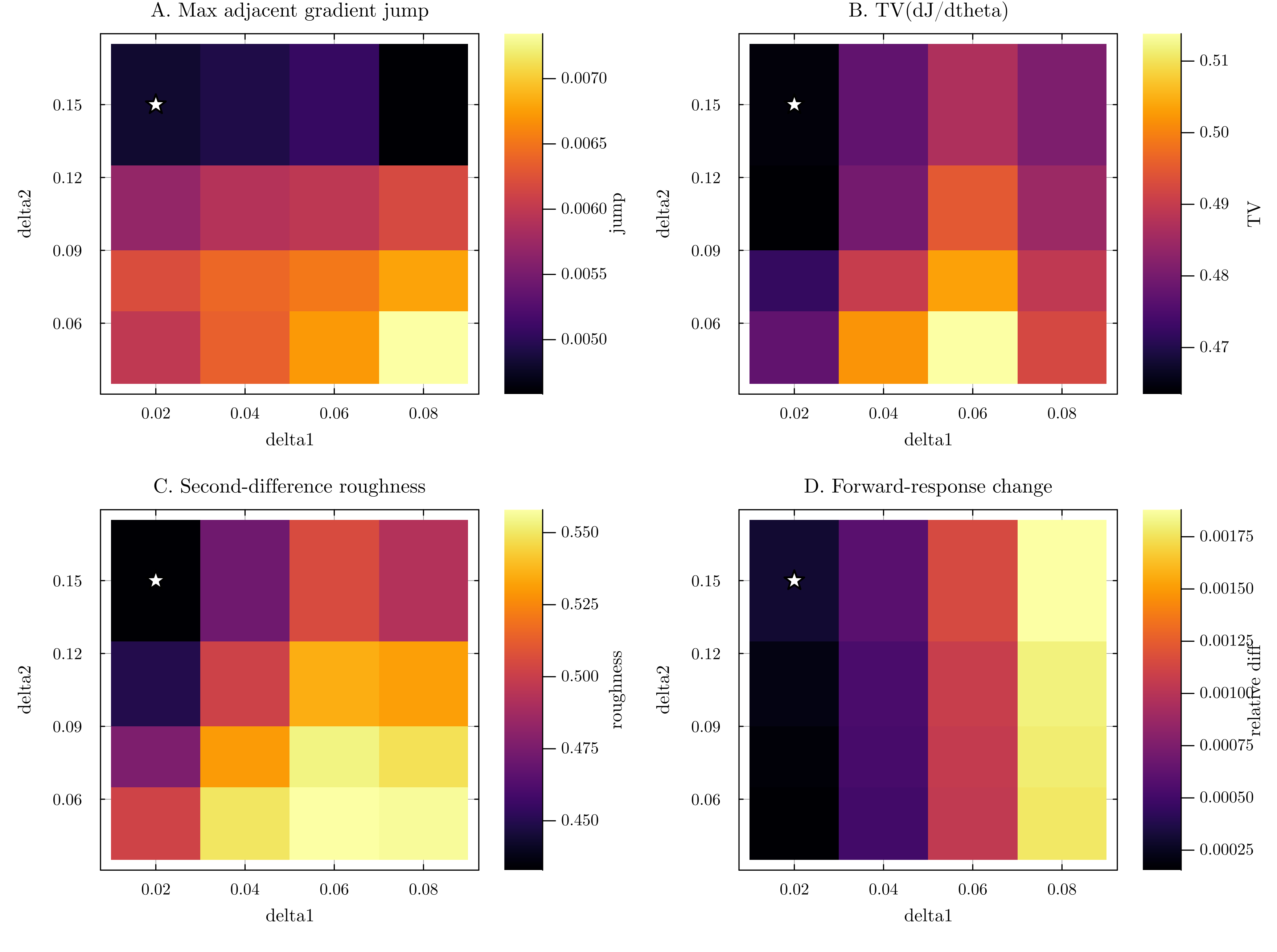
In this diagnostic, increasing delta2, the width of the upper transition around r = 5/2, gives the clearest reduction in sensitivity roughness. Increasing delta1, the width around r = 1/4, does not improve the metrics as consistently and tends to increase the forward-response change. The best tested point by second-difference roughness is
\[\delta_1 = 0.02,\qquad \delta_2 = 0.15.\]
This candidate reduces the second-difference roughness from about 0.502 for the current regularised setting (delta1, delta2) = (0.02, 0.05) to about 0.433, while keeping the maximum relative forward-response change small, about 3.0e-4. This suggests that widening only the upper Koren transition may be a useful future tuning direction, but the current production values remain the conservative default until broader validation is performed.
Structured parameter sweep
The repository also includes a structured TVD sweep over
delta0 in {0.005, 0.01, 0.02, 0.04}delta1 in {0.005, 0.01, 0.02, 0.04}delta2 in {0.02, 0.05, 0.08, 0.12}
for a total of 64 checked parameter combinations.
From the checked-in tvd_sweep_results.csv and the rerun of sweep_tvd_safety.jl:
64 / 64configurations satisfy the geometry constraints64 / 64pass the analytic TVD certificate64 / 64pass the dense-grid TVD check
Within this sweep envelope, the retained cubic-Hermite smoothing widths remain TVD-safe. Since the r = 0 patch is disabled, delta0 no longer affects the active production limiter; it is retained only for compatibility with older sweep files and validation configurations.
Why this case matters
- It isolates the smoothed nonlinear piece introduced for differentiability in the explicit solver.
- It guards against future edits that could preserve
C1smoothness but violate TVD admissibility. - It complements the full-model gradient experiments by showing that the limiter itself is not the weak link at the retained branch transitions.
- It documents the accuracy/smoothness tradeoff: very smooth gradients can be obtained with upwind diffusion, but the regularised Koren diagnostic achieves lower gradient roughness with negligible forward-response change.
How to run
Scripts
Folder: validation/TVD_limiter
Core implementation:
validation/TVD_limiter/tvd_limiter_common.jl
Drivers:
validation/TVD_limiter/test_tvd_limiter.jlvalidation/TVD_limiter/test_tvd_limiter_strong.jlvalidation/TVD_limiter/sweep_tvd_safety.jlvalidation/TVD_limiter/regularised_koren_diagnostic.jl
Run
julia --project=. validation/TVD_limiter/test_tvd_limiter.jl
julia --project=. validation/TVD_limiter/test_tvd_limiter_strong.jl
julia --project=. validation/TVD_limiter/sweep_tvd_safety.jl
julia --project=. validation/TVD_limiter/regularised_koren_diagnostic.jl
Outputs
The tests primarily report to standard output. The structured sweep writes:
validation/TVD_limiter/tvd_sweep_results.csv
The source-position diagnostic writes:
validation/TVD_limiter/out/limiter_gradient_noise_tradeoff.pngvalidation/TVD_limiter/out/limiter_gradient_noise_tradeoff.pdfvalidation/TVD_limiter/out/data/limiter_gradient_noise_tradeoff_metrics.csv- additional limiter, local-stencil, and sensitivity-sweep CSV/figure files under
validation/TVD_limiter/out/
Notes
- The certificate is numerical, not symbolic: it is stronger than brute-force sampling on each cubic patch, but it is not a formal theorem prover.
- TVD safety is therefore a validated property of the checked parameter sets, not an automatic guarantee for arbitrary Hermite widths.
- The sensitivity diagnostic is comparative and grid-dependent. It should be used to support the narrower claim that the retained regularisation reduces limiter-induced gradient noise in the tested plume response, not to claim global differentiability of the full model.