Gradient / AD experiments
Purpose
These experiments validate the gradient pathways used in inversion-oriented TARSA workflows. They answer four practical questions:
- Are the implemented gradients numerically consistent with finite differences?
- How expensive are different gradient engines relative to one forward run?
- Do limiter non-smoothness and CFL choices break gradient agreement?
- Can the gradients drive small inverse problems for emissions and nonlinear parameters?
Most experiments use a shared synthetic Gaussian transport testbed, then change only the control parameter, observation operator, or optimization loop.
Common setup
The shared implementation lives in:
validation/GRADIENTS/experiment_gradcheck_gaussian_adfull.jl
Most experiments use a small 3-D Gaussian plume configuration with:
- uniform along-wind advection
- explicit DST-Koren transport
- implicit vertical diffusion
- synthetic observations sampled either at point receptors or through a simple AOD-like operator
- least-squares objectives built from forward-model output
The experiments vary the control variable:
- scalar emission scale $\alpha$
- time-binned emission scaling factors
- nonlinear loss-rate scaling
- AOD-observation variants of the same nonlinear inversion
Gradient definitions
For the core scalar test, the control is an emission multiplier $\alpha$ applied to a fixed source pattern $E_0$, so
\[E(\alpha) = \alpha E_0.\]
The discrete one-step update is viewed in affine form as
\[\mathbf{X}^{n+1} = \mathbf{A}_{\mathrm{step}}\,\mathbf{X}^n + \mathbf{q}(\theta),\]
where $\theta$ denotes the control vector and $\mathbf{q}(\theta)$ collects the control-dependent source or boundary contribution. In the minimal scalar experiment, $\theta = \alpha$ and the transport operators are fixed, so the forward model is affine in $\alpha$.
The observation operator $H$ maps the model state into the sampled receptor/time space used by the least-squares objective:
\[J(\alpha)=\frac12\bigl(HX(\alpha)-y\bigr)^{\mathrm T}\mathbf{R}^{-1}\bigl(HX(\alpha)-y\bigr),\]
with $\mathbf{R}=\mathbf{I}$ in this minimal experiment. For notational convenience, we can still write the sampled model vector as
\[m(\alpha) = HX(\alpha), \qquad r(\alpha)=HX(\alpha)-y.\]
The independent finite-difference reference used throughout Experiment 1 is
\[g_{\mathrm{FD}}(\varepsilon)=\frac{J(\alpha_0+\varepsilon)-J(\alpha_0-\varepsilon)}{2\varepsilon},\]
evaluated here at $\alpha_0 = 0.9$.
Analytical gradient
In Experiment 1 the source scaling is linear and all operators are fixed, so the sampled model response is affine in $\alpha$:
\[HX(\alpha)=HX(0)+\alpha\,HX(1).\]
Therefore the exact scalar gradient used by the analytic method is
\[\frac{\mathrm{d}J}{\mathrm{d}\alpha} = \bigl(HX(\alpha_0)-y\bigr)^{\mathrm T}\mathbf{R}^{-1}HX(1).\]
This is the logic implemented through precompute_emiss_response(...) and the grad_mode=:analytic branch in experiment_gradcheck_gaussian_adfull.jl, where the repository computes
\[m^{(1)} = HX(1)-HX(0)\]
from two forward runs and then contracts that sampled response with the residual.
Tangent gradient
The tangent-linear equation is
\[\mathbf{S}^{n+1} = \mathbf{A}_{\mathrm{step}}\,\mathbf{S}^{n} + \frac{\partial \mathbf{q}}{\partial \alpha},\]
where
\[\mathbf{S}^n = \frac{\partial \mathbf{X}^n}{\partial \alpha}.\]
After mapping the tangent state into observation space, the gradient is
\[\frac{\mathrm{d}J}{\mathrm{d}\alpha} = \bigl(HX(\alpha_0)-y\bigr)^{\mathrm T}\mathbf{R}^{-1} H S.\]
This is the tangent method implemented with TARSA.advect_dst_koren_dimsplit_tangent! plus a tangent solve through the vertical-diffusion step. In the repository code, $HS$ is assembled by sampling the propagated tangent state at the same receptors and times as the forward trajectory.
Adjoint gradient
The adjoint is the discrete adjoint associated with the transpose of the one-step operator. Written in observation-sampled form, a consistent backward sweep is
\[\boldsymbol{\lambda}^{n} = \mathbf{A}_{\mathrm{step}}^{\mathrm T}\boldsymbol{\lambda}^{n+1} + \mathbf{H}_n^{\mathrm T}\mathbf{R}_n^{-1}\bigl(\mathbf{H}_n\mathbf{X}^n-\mathbf{y}_n\bigr),\]
with one residual injection term whenever an observation is present at time level $n$. The scalar gradient is then accumulated as
\[\frac{\mathrm{d}J}{\mathrm{d}\alpha} = \sum_n \left(\frac{\partial \mathbf{q}^n}{\partial \alpha}\right)^{\mathrm T}\boldsymbol{\lambda}^{n+1}.\]
For the Gaussian scalar-source test, $\partial \mathbf{q}^n / \partial \alpha$ is just the fixed emission pattern inserted at each substep, so the implementation reduces to accumulating its inner product with the backward variable. This matches the code path in loss_grad_alpha_koren_dimsplit(...), where the source contribution appears as sum(lambda_phi_star .* (dt_sub .* cfg.emiss_base)).
Autodiff backend
The autodiff backend is implemented with ForwardDiff.jl:
- scalar controls use
ForwardDiff.derivative(f, alpha) - vector controls use
ForwardDiff.gradient(f, alpha_vec)
So in Experiment 1 the autodiff column is the forward-mode ForwardDiff.jl derivative of the full scalar loss function $f(\alpha)=J(\alpha)$. The separate Enzyme-based scripts remain supplementary checks and are listed explicitly below.
Results
Experiment 1: gradient agreement and finite-difference U-curve
This is the core scalar gradient check. It compares analytic, tangent, autodiff, and adjoint gradients against centered finite differences in Float32. Here autodiff specifically means the ForwardDiff.jl forward-mode derivative of the scalar loss function.
Runtime figure: 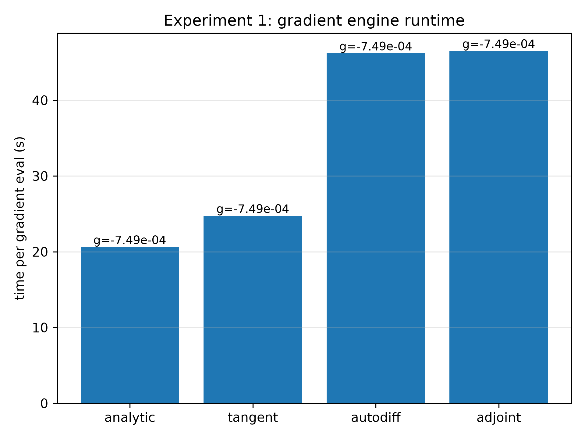
U-curve figure: 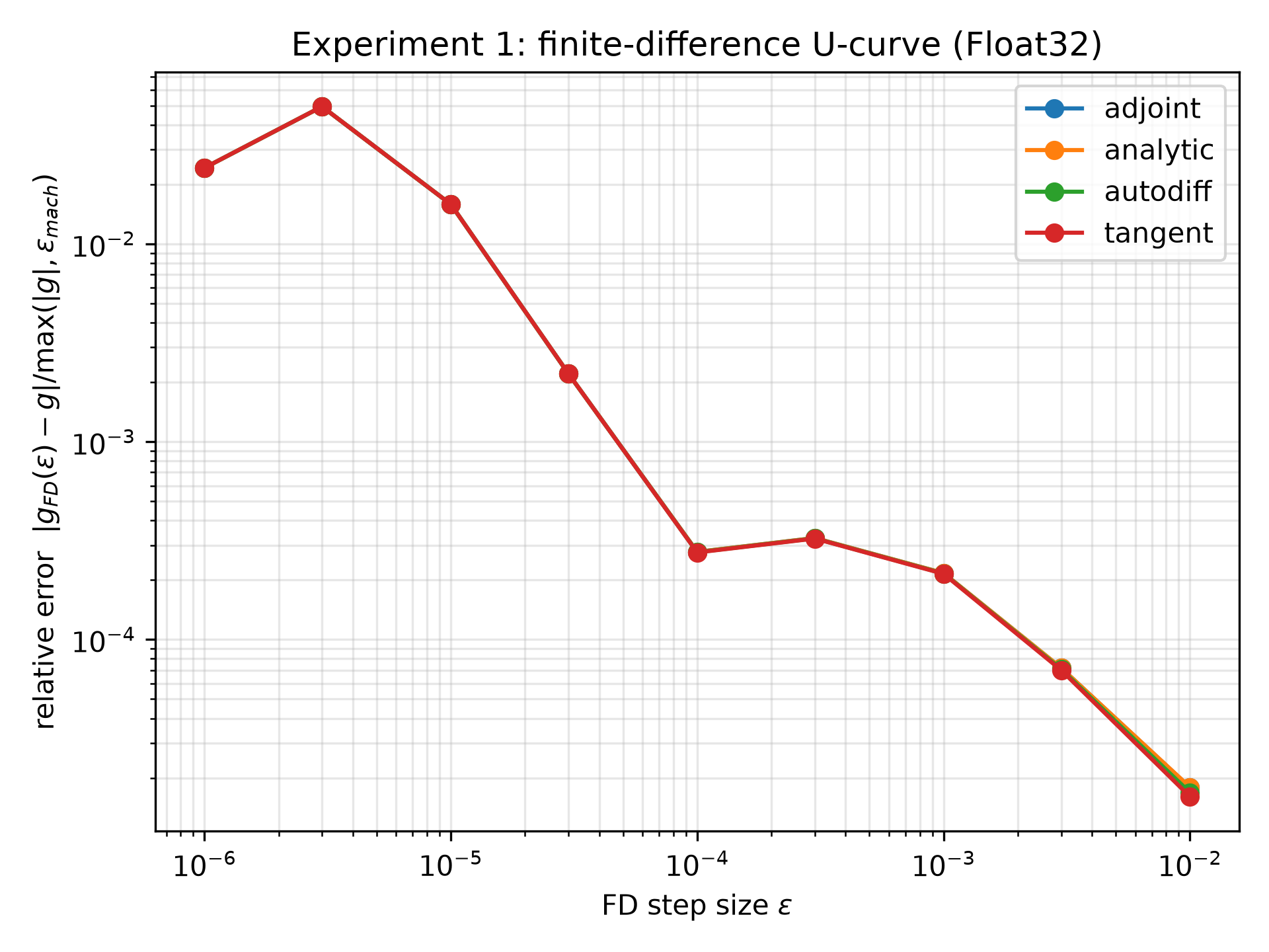
The main result is that the analytic, tangent, autodiff, and adjoint gradients all agree very well with centered finite differences in this scalar check.
Representative metrics from the checked-in summary:
| Method | Time (s) | Best FD step | Best relative error |
|---|---|---|---|
| analytic | 20.634 | 1e-2 | 1.794e-5 |
| tangent | 24.753 | 1e-2 | 1.608e-5 |
| autodiff | 46.209 | 1e-2 | 1.686e-5 |
| adjoint | 46.516 | 1e-2 | 1.787e-5 |
Interpretation:
- analytic and tangent gradients are essentially identical in this scalar test
- forward-mode autodiff is slower but reaches the same accuracy range
- the adjoint is as accurate as the other engines here (best rel. err.
1.787e-5, matching the analytic gradient to ~7 digits) - the U-curve behaves as expected: too-large and too-small finite-difference steps both degrade agreement
Experiment 2: gradient cost scaling
This experiment compares gradient cost to forward cost as the problem size grows.
Cost-ratio figure: 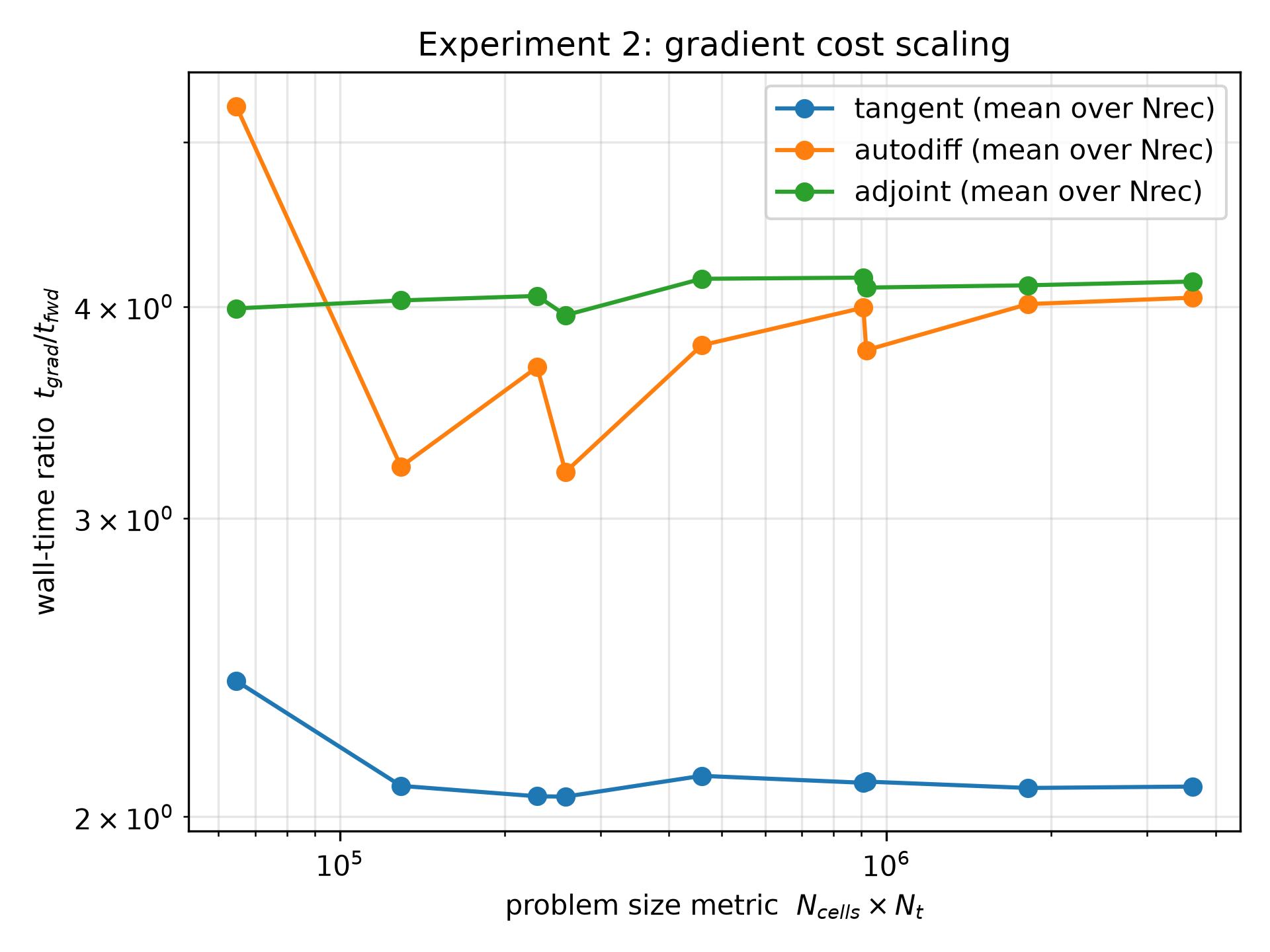
Wall-time figure: 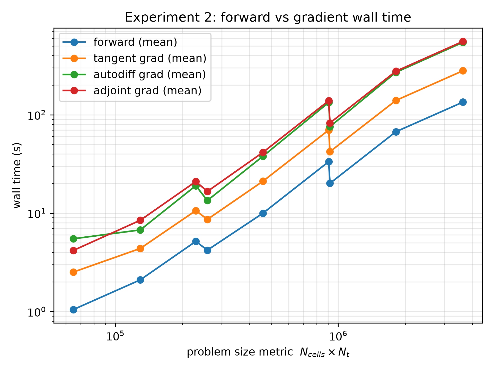
The ratio plot is the more stable summary. At the largest tested size metric N_cells x N_t = 3,628,800, the mean gradient-to-forward wall-time ratios are approximately:
- tangent:
2.08x - autodiff:
4.05x - adjoint:
4.14x
Interpretation:
- tangent mode is the cheapest gradient engine in this tested regime
- autodiff is consistently more expensive than tangent but cheaper than adjoint
- adjoint cost is fairly flat in ratio space here, around
4xthe forward cost - absolute times increase with problem size for all methods, but the ordering remains stable
Experiment 3: limiter non-smoothness stress test
experiment3.jl sweeps advect_tiny, advect_cfl, and noise levels to check whether the Koren limiter causes catastrophic finite-difference disagreement.
There is no checked-in figure for this experiment, but the summary numbers are reassuring:
- worst best relative error at
0 %noise:1.317e-5 - worst best relative error at
1 %noise:1.294e-5 - both worst cases occur at
CFL = 0.50(attiny = 1e-8and1e-12, respectively)
Interpretation:
- in the tested range, limiter non-smoothness does not destroy gradient agreement
- finite-difference agreement remains in the low-
1e-5range even when small observation noise is added
Experiment 4: inversion of time-binned emissions
This experiment promotes the scalar control to a vector of emission-scale factors, one per time bin.
Convergence figure: 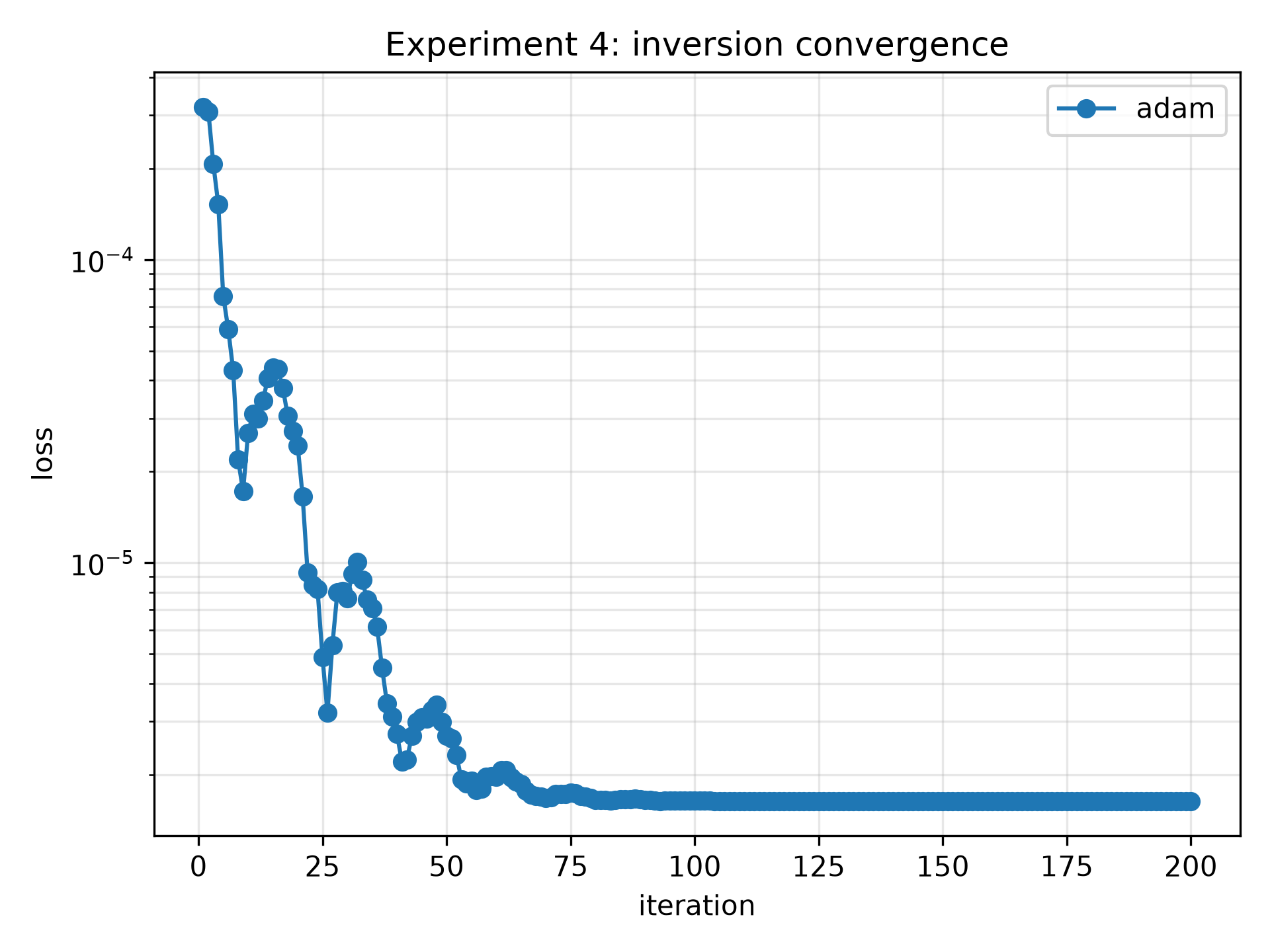
Recovery figure: 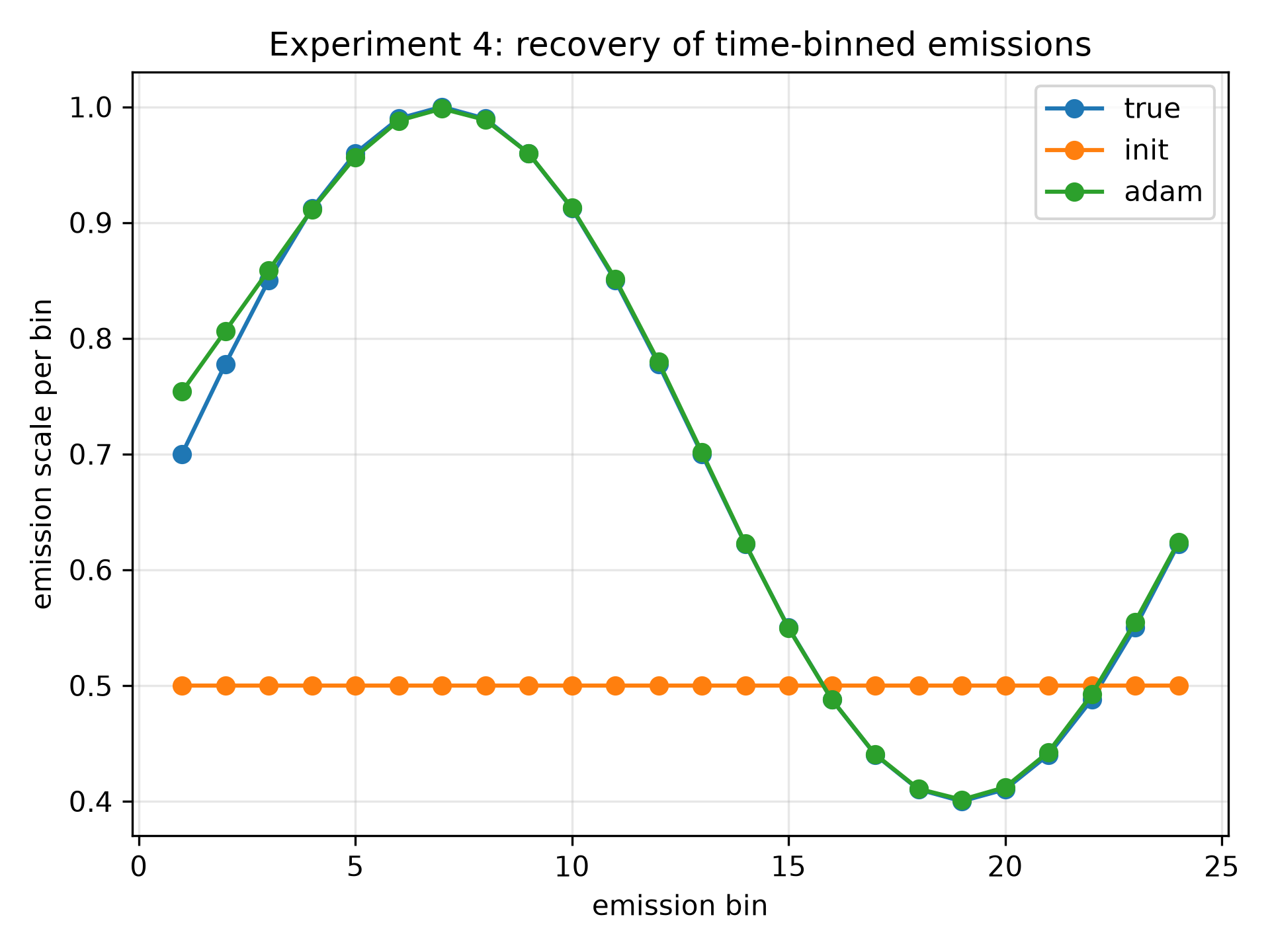
The result is visually clear:
- the Adam-based inversion rapidly reduces the loss by roughly two orders of magnitude
- plain gradient descent stays close to the initial guess and barely recovers the true structure
- Adam recovers the full time-binned emission pattern almost on top of the truth
Representative recovery metrics from the checked-in summary:
- Adam RMSE on recovered bin scales:
1.272e-2 - Adam correlation with truth:
0.998
Interpretation:
- the gradients are good enough to recover a multi-parameter emission profile, not just a scalar
- optimizer choice matters strongly: the same gradients that work well with Adam are ineffective with the naive gradient-descent setup used here
Experiment 5: inversion of nonlinear loss-rate scale
This experiment estimates a scalar multiplier on the loss field,
\[\lambda(\alpha) = \alpha \lambda_0(x,y,z),\]
so the control parameter affects the model dynamics at every step.
Recovered-alpha figure: 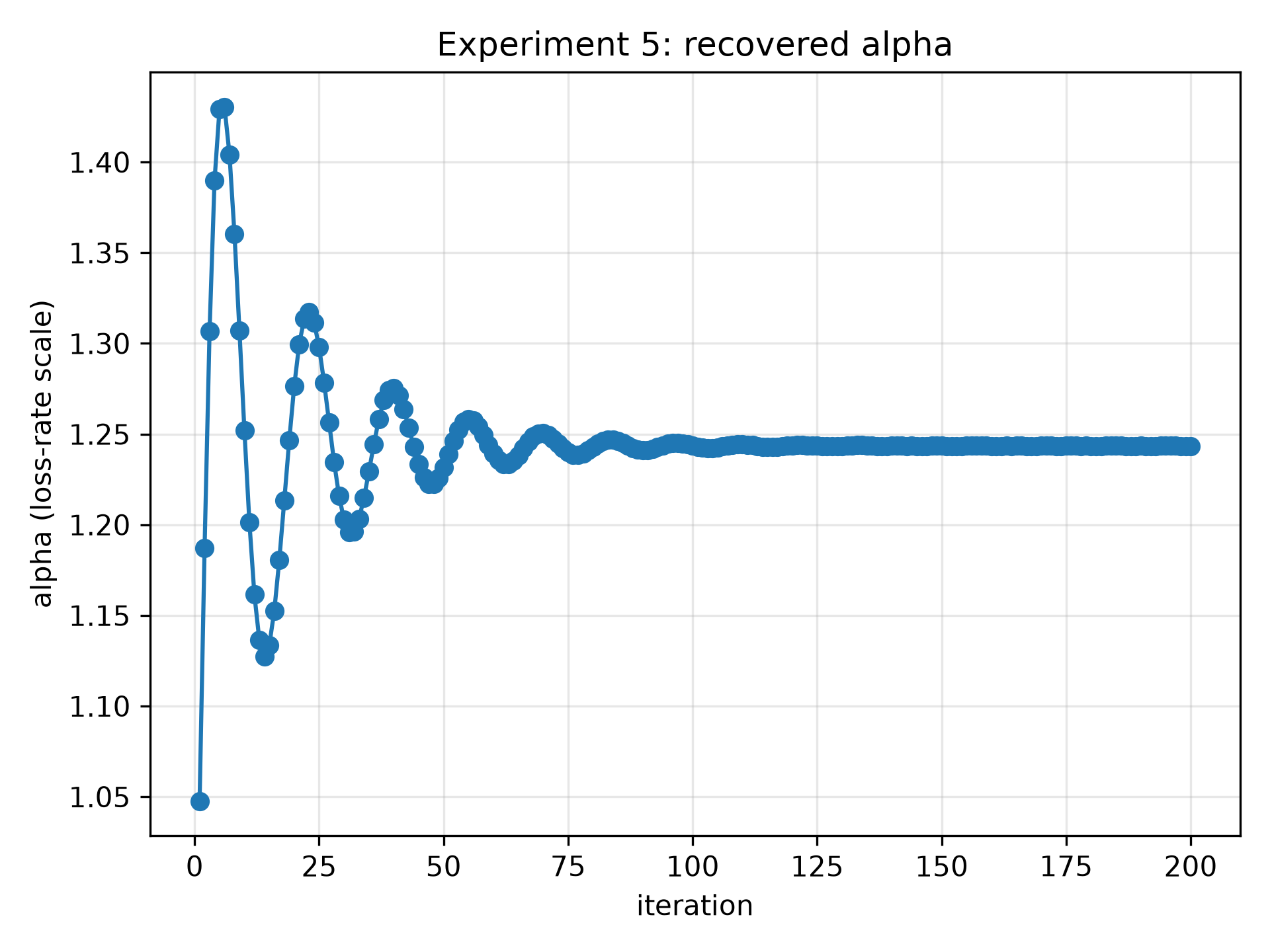
Convergence figure: 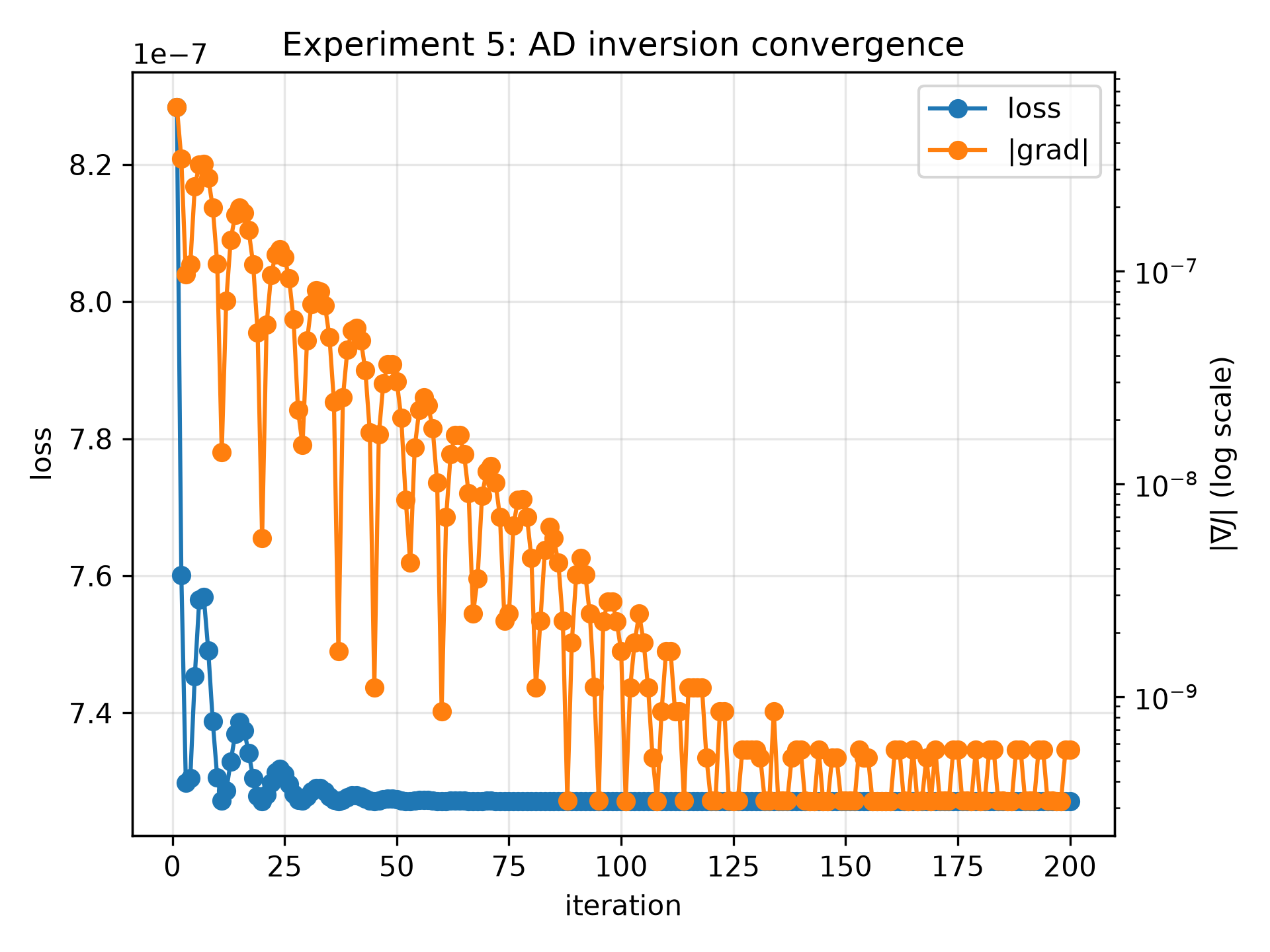
In this case the goal is to show that TARSA can differentiate through a genuinely nonlinear parameterized process, not just through a linear source scaling.
Important nuance for the checked-in outputs:
- the optimization starts at
alpha = 0.9withalpha_true = 1.2 - the Adam path (
experiment5_ad_convergence.csv) settles nearalpha = 1.243 - the separate LM run (
experiment5_lm_convergence.csv) converges to the same value,alpha = 1.243 - the minimum reported loss is
7.271e-7
Interpretation:
- the experiment demonstrates that the nonlinear-loss gradient is usable: both optimizers drive the loss to its
~7.27e-7floor - both runs settle near
alpha = 1.243, a small overshoot of the true1.2; two independent optimizers landing on the same value indicates this offset is the discretized loss minimum, not an optimizer artifact - the figure should be read as an optimization-path diagnostic, with the residual offset from
alpha_truereflecting that shallow minimum
Additional scripts
Two additional experiment scripts are part of the folder even though they do not currently have checked-in figures on this docs page:
experiment_gradcheck_gaussian_enzyme_rk3.jlRepeats the scalar gradient check using Enzyme on the RK3 Gaussian configuration. This is separate from the mainautodiffmethod above, which usesForwardDiff.jl.
Why this case matters
- validates the gradient engines needed for future inverse and assimilation workflows
- quantifies the runtime trade-off between tangent, autodiff, and adjoint approaches
- checks that limiter non-smoothness does not invalidate gradient-based use of the explicit solver
- shows that TARSA gradients can support both scalar and multi-parameter inverse problems
How to run
Scripts
Folder: validation/GRADIENTS
Core shared implementation:
validation/GRADIENTS/experiment_gradcheck_gaussian_adfull.jl
Experiment drivers:
validation/GRADIENTS/experiment1_ucurve.jlvalidation/GRADIENTS/experiment2.jlvalidation/GRADIENTS/experiment3.jlvalidation/GRADIENTS/experiment4.jlvalidation/GRADIENTS/experiment4ad.jlvalidation/GRADIENTS/experiment5.jlvalidation/GRADIENTS/experiment_gradcheck_gaussian_enzyme_rk3.jl
Helpers:
validation/GRADIENTS/plot_grad_experiments.pyvalidation/GRADIENTS/gradient_experiments_summary.tex
Representative CSV outputs:
validation/GRADIENTS/experiment1_ucurve_methods.csvvalidation/GRADIENTS/experiment1_ucurve_fdcurve.csvvalidation/GRADIENTS/experiment2_scaling.csvvalidation/GRADIENTS/experiment3_nonsmooth.csvvalidation/GRADIENTS/experiment4_mininv_timeseries.csvvalidation/GRADIENTS/experiment4_mininv_convergence.csvvalidation/GRADIENTS/experiment4ad_mininv_timeseries.csvvalidation/GRADIENTS/experiment4ad_mininv_convergence.csvvalidation/GRADIENTS/experiment5_ad_convergence.csvvalidation/GRADIENTS/experiment5_lm_convergence.csv
Run
julia --project=. validation/GRADIENTS/experiment1_ucurve.jl
julia --project=. validation/GRADIENTS/experiment2.jl
julia --project=. validation/GRADIENTS/experiment3.jl
julia --project=. validation/GRADIENTS/experiment4.jl
julia --project=. validation/GRADIENTS/experiment5.jl
python validation/GRADIENTS/plot_grad_experiments.py
Notes
- The main
autodiffbackend on this page isForwardDiff.jl:ForwardDiff.derivativefor scalar controls andForwardDiff.gradientfor vector controls. Enzyme.jlis only used in the supplementary Enzyme-specific scripts, not in the mainautodiffrows of Experiments 1 and 2.plot_grad_experiments.pyis the source of the checked-in figures underdocs/src/img/figures_for_gradients/.- These are computational experiments, so runtimes depend strongly on problem size and chosen backend.